denoisingCTF Tutorial
tutorial.RmdThis tutorial will guide you through the usage of the main functions of the package. You can either use the function rm_noise to remove the noise applying the current trained models, or train your own models and then call them into the main function.
Getting started
You will need to install the devtools CRAN package. All other dependencies will be automatically installed with the package installation.
# Install devtools
install.packages("devtools")

# Install denoisingCTF
devtools::install_github("msenosain/denoisingCTF")
Preparing your data
Before you attempt to clean your data or train your own models, your FCS files should be previously normalized using a bead normalization software. Additionally, for your files to be comparable they must have the same antibody panel which means same number of channels with same names and descriptions. Both can be done using the premessa package (See functions paneleditor_GUI and normalizer_GUI).
Denoising CyTOF data
The rm_noise function will remove zeros, beads and debris from the FCS files in the current working directory using previously trained models.
denoisingCTF::rm_noise()After printing the list of column names with the index number, a first prompt will ask the user for the “mandatory” markers, which can be any marker that should be expressed in the cells (e.g. post-fixation DNA intercalator).
## Warning in readFCSdata(con, offsets, txt, transformation, which.lines, scale, : Some data values of 'Time' channel exceed its $PnR value 6076541 and will be truncated!
##  To avoid truncation, either fix $PnR before generating FCS or set 'truncate_max_range = FALSE'
## Warning in readFCSdata(con, offsets, txt, transformation, which.lines, scale, : Some data values of 'Event_length' channel exceed its $PnR value 50 and will be truncated!
##  To avoid truncation, either fix $PnR before generating FCS or set 'truncate_max_range = FALSE'
##       [,1]
##  [1,] "Time_Time"
##  [2,] "Event_length_Event_length"
##  [3,] "Pd102Di_102Pd"
##  [4,] "Rh103Di_103Rh"
##  [5,] "Pd104Di_104Pd"
##  [6,] "Pd105Di_105Pd"
##  [7,] "Pd106Di_106Pd"
##  [8,] "Pd108Di_108Pd"
##  [9,] "Pd110Di_110Pd"
## [10,] "Sn120Di_120Sn"
## [11,] "I127Di_127I"
## [12,] "Xe131Di_131Xe"
## [13,] "Cs133Di_133Cs"
## [14,] "Ce140Di_140Ce"
## [15,] "Pr141Di_141Pr_EpCAM"
## [16,] "Ce142Di_142Ce"
## [17,] "Nd142Di_142Nd_ccasp3"
## [18,] "Nd143Di_143Nd_TP53"
## [19,] "Nd144Di_144Nd_HLA-ABC"
## [20,] "Nd145Di_145Nd_CD31"
## [21,] "Nd146Di_146Nd_Thioredoxin"
## [22,] "Sm147Di_147Sm_b-CAT"
## [23,] "Nd148Di_148Nd_HER2"
## [24,] "Sm149Di_149Sm_p-STAT6"
## [25,] "Nd150Di_150Nd_p-STAT5"
## [26,] "Eu151Di_151Eu_TTF1"
## [27,] "Sm152Di_152Sm_p-AKT"
## [28,] "Eu153Di_153Eu_Ki67"
## [29,] "Sm154Di_154Sm_CD45"
## [30,] "Gd155Di_155Gd_CD56"
## [31,] "Gd156Di_156Gd_Vimentin"
## [32,] "Gd157Di_157Gd"
## [33,] "Gd158Di_158Gd_p-STAT3"
## [34,] "Tb159Di_159Tb_CD4"
## [35,] "Gd160Di_160Gd_MDM2"
## [36,] "Dy160Di_160Dy"
## [37,] "Dy161Di_161Dy_Cytokeratin"
## [38,] "Dy162Di_162Dy_MET"
## [39,] "Dy163Di_163Dy_TP63"
## [40,] "Dy164Di_164Dy_CK7"
## [41,] "Ho165Di_165Ho_EGFR"
## [42,] "Er166Di_166Er_CD44"
## [43,] "Er167Di_167Er_p-ERK"
## [44,] "Er168Di_168Er_CD8"
## [45,] "Tm169Di_169Tm_CD24"
## [46,] "Yb170Di_170Yb_CD3"
## [47,] "Yb171Di_171Yb_CD11b"
## [48,] "Yb172Di_172Yb_p-S6"
## [49,] "Yb173Di_173Yb_CD90"
## [50,] "Yb174Di_174Yb_HLA-DR"
## [51,] "Lu175Di_175Lu_PD-L1"
## [52,] "Yb176Di_176Yb_His-H3"
## [53,] "Hf178Di_178Hf"
## [54,] "Hf179Di_179Hf"
## [55,] "Hf180Di_180Hf"
## [56,] "Ta181Di_181Ta"
## [57,] "W182Di_182W"
## [58,] "W183Di_183W"
## [59,] "W184Di_184W"
## [60,] "Re185Di_185Re"
## [61,] "Os186Di_186Os"
## [62,] "Re187Di_187Re"
## [63,] "Os188Di_188Os"
## [64,] "Os189Di_189Os"
## [65,] "BCKG190Di_190BCKG"
## [66,] "Ir191Di_191Ir"
## [67,] "Os192Di_192Os"
## [68,] "Ir193Di_193Ir"
## [69,] "Pt194Di_194Pt"
## [70,] "Pt195Di_195Pt"
## [71,] "Pt198Di_198Pt"
## [72,] "Pb208Di_208Pb"
## [73,] "Center_Center"
## [74,] "Offset_Offset"
## [75,] "Width_Width"
## [76,] "Residual_Residual"
## [77,] "beadDist_beadDist"
## Enter the column INDICES of the 'mandatory' markers (separated by single space only, no comas allowed)
Any cell/event/row that has zero expression of this marker is removed. In this example our “mandatory” marker is Histone H3:
##[52,] "Yb176Di_176Yb_His-H3"
A second prompt will ask the user for the “optional” markers, which can be markers used for cell type identification.
## Enter the column INDICES of the 'optional' markers (separated by single space only, no comas allowed)Any cell/event/row that has zero expression of all this markers, meaning that it cannot be identified as any existing cell type, is removed. In this example our “optional” markers are the following:
## [15,] "Pr141Di_141Pr_EpCAM"## [20,] "Nd145Di_145Nd_CD31"## [29,] "Sm154Di_154Sm_CD45"## [31,] "Gd156Di_156Gd_Vimentin"## [34,] "Tb159Di_159Tb_CD4"## [37,] "Dy161Di_161Dy_Cytokeratin"## [40,] "Dy164Di_164Dy_CK7"## [44,] "Er168Di_168Er_CD8"## [46,] "Yb170Di_170Yb_CD3"## [47,] "Yb171Di_171Yb_CD11b"## [49,] "Yb173Di_173Yb_CD90"
The next prompt will ask the user for the beads channels column indices, and the last prompt will ask for the Gaussian parameters channels and the intact-cells marker channel. The latter could be any marker used to distinguish dead cells from live cells, such as a DNA intercalator post-fixation (e.g. iridium) or an antibody for DNA protein (e.g. Histone H3). This will be used as input features for the beads model and the debris model, respectively. Events classified as beads or debris will be removed.
## Enter the column INDICES of the beads channels Ce140, Eu151, Eu153, Ho165, Lu175 (separated by single space only, no comas allowed)## Enter the column INDICES of the gaussian parameters channels 'Event_length', 'Center', 'Offset', 'Residual', 'Width' and intact-cells marker channel (separated by single space only, no comas allowed)Finally, this function will create a new directory called output which will contain the newly written FCS files after noise removal. Additionally, within the output folder you will find a folder called noiseCL containing CSV files with the original data and the added columns beads and debris in which 0 means negative and 1 means positive for beads/noise (0 could be interpreted as ‘cells’). The user can use the CSV files to assess the accuracy of the classification if needed.
See below for an example of the output’s directory structure:
## .
## ├── 181018_2_11841_PX_normalized.fcs
## ├── 181018_4_13651_I_normalized.fcs
## ├── 181018_6_13074_P_normalized.fcs
## ├── 181019_0_normalized.fcs
## ├── 181019_1_11817_P_normalized.fcs
## └── output
##     ├── 181018_2_11841_PX_normalized_denoised.FCS
##     ├── 181018_4_13651_I_normalized_denoised.FCS
##     ├── 181018_6_13074_P_normalized_denoised.FCS
##     ├── 181019_0_normalized_denoised.FCS
##     ├── 181019_1_11817_P_normalized_denoised.FCS
##     └── noiseCL
##         ├── 181018_2_11841_PX_normalized_noiseCL.csv
##         ├── 181018_4_13651_I_normalized_noiseCL.csv
##         ├── 181018_6_13074_P_normalized_noiseCL.csv
##         ├── 181019_0_normalized_noiseCL.csv
##         └── 181019_1_11817_P_normalized_noiseCL.csv
Model training
The rm_noise function can take new models as input in the arguments model_beads and model_debris when use.current.model.beads=FALSE and use.current.model.debris=FALSE, respectively. In this section, you will see step by step how can you build training and test data sets and train new models.
I would advise to always train and use your own models because these may be sensible to bead normalization. Also, because: * you may have a different strategy to identify debris and dead cells. * you may have used a different set of normalization beads.
Beads model
1. Build training and test datasets You should set up your working directory to the folder that contains your FCS files of interest.
setwd("~/Documents/My_CyTOF_Files")The Beads_TrainTest function will select a random sample from your FCS files (length specified in sample_size argument), and a promt will ask the user for the beads channels column indices.
denoisingCTF::Beads_TrainTest(sample_size = 20, method = 'k_means',
    bsample = 5000, class_col = 'BeadsSmp_ID', ...)
## Enter the column INDICES of the beads channels (separated by single space only, no comas allowed)Then it will apply arcsinh tranformation (cofactor=5) and perform an unsupervised detection of the beads using a clustering method, which can be either by k-means or Gaussian Mixture Models. Clustering results will be evaluated and only the files in which the events identified as beads show a coefficient of variation (CV) <0.05 will be selected to be part of the training and test sets. In all cases, the function writes a CSV file with the summary statistics, labeled filename_beadsstats.csv for a file that passed the test, or filename__FAILEDbeadsstats.csv for a file in which the clustering failed to identify the beads correctly.
Since CyTOF experiments usually render a large number of events (sometimes more than a million) and we do not need that many events to train a model; the function will take a random sample of the files for which the clustering was successful. This will be a balanced sample, having bsample number of events per class. If bsample is larger than the amount of events available for that class then replacement=TRUE.
From the n ‘good’ files, 0.75 will be randomly pulled for the training set and the remaining 0.25 will be the test set (default). The proportion can be changed by passing the argument s_train, which determines the size of the fraction that goes into the training set (any number between 0:1).
Finally, the function writes a .RData file that includes:
-
train_set: adata.framewith the training set. -
test_set: adata.framewith the test set. -
train_nms: a character vector with the names of the files used as they appear intrain_set. Can be interpreted as row names oftrain_set. -
test_nms: a character vector with the names of the files used as they appear intest_set. Can be interpreted as row names oftest_set.
2. Model training To train the new beads model use the TrainModel function. You can specify which algorithm to use in the argument alg (see documentation) for details).
denoisingCTF::TrainModel(train_set, test_set, alg = 'all', class_col = 'BeadsSmp_ID',
    seed = 40, name_0 = 'cells', name_1 = 'beads', label = 'beads',
    allowParallel = T, free_cores = 2)
This function will write a .RData file that includes:
-
model_alg: the trained model. -
ftimp_alg: feature importance. -
pred_alg: the predicted classes for the test set. -
conf_alg: the confusion matrix from the test set prediction.
Debris model
1. Build training and test datasets
The function pre_gate will preprocess the data by:
- Removing zeros (as explained above for ‘mandatory’ and ‘optional’ markers)
- Removing beads (using beads model)
- Adding a row ID column
denoisingCTF::pre_gate(sample_size=30, model_beads=model_beads, alg_bd = 'RF')The function will write new FCS files in a folder called ‘toy_debris’. The user will then use their preferred strategy to “gate out” the debris and dead cells. Here we used Fluidigm recommendations and our marker for intact cells:
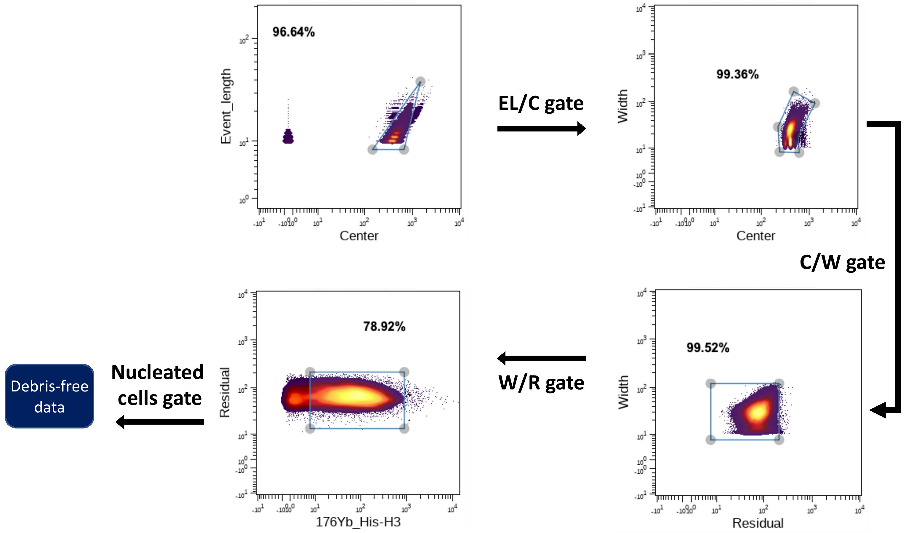
Manual gating example
Once that is done, download your gated files (noise is already removed) into a new folder inside the ‘toy_debris’ directory. The post_gate function will compare pre- and post-gated files, label noise and generate training and test datasets. As explained above, bsample is the size of the random sample to be taken from each class. The function will write a .RData file with the same content explained above, but this time the class column will be named GP_Noise.
denoisingCTF::post_gate(bsample = 5000, path_pregated = '../') 2. Model training
This is exactly the same as for the beads model training but using as training features the channels you used to gate the noise out and changing some labels:
denoisingCTF::TrainModel(train_set, test_set, alg = 'all', class_col = 'GP_Noise',
    seed = 40, name_0 = 'cells', name_1 = 'debris', label = 'debris',
    allowParallel = T, free_cores = 2)